Quickstart: Python API

Background. Habitat analysis splits a tumour into sub-regions that behave alike across the input images (here, DCE phases), then describes each tumour by how much of each sub-region it has and how they are arranged.

Purpose. You get your first habitat maps, a per-subject feature table (volume fractions, MSI, ITH, graph), and a saved model that labels a new patient without refitting.

Key terms.

• habitat – a sub-region inside the tumour (the ROI) whose voxels behave alike across the input images; HABIT paints each ROI voxel with a habitat id (1, 2, 3, …).

• ROI / mask – the region of interest, usually the whole tumour, stored as an integer mask; only voxels inside it are analysed (0 = background).

• voxel feature – the numbers that describe one voxel (here its intensity in each DCE phase); one column per feature.

• supervoxel – a small patch of neighbouring voxels with similar features, clustered inside one subject first (partition), so the cohort model clusters tens of rows per subject instead of every voxel.

• pool – stacks every training subject’s rows into one matrix so one model is fitted to the whole cohort and habitat ids mean the same thing in every patient.

• fit – learns the habitat definition (for k-means: the number of habitats and their centroids).

• assign – gives every supervoxel / voxel the id of its nearest centroid, producing the habitat map.

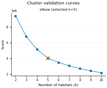
• Stage / Spec / HabitatSpec – a Stage is one step with a label you choose; a Spec names a registered component and its parameters; a HabitatSpec is the ordered list of stages plus random_seed, i.e. the whole study definition.

• elbow – a rule for picking the number of habitats: the candidate count after which adding one more habitat stops reducing within-cluster spread much.

A short list of stages declares the analysis; one call fits it on a cohort. Everything after that is looking at the result: the habitat map, the per-habitat features a paper would report, and reusing the fitted model on a new patient. No YAML.

Install first (Installation). This page uses the official demo pack (five liver lesions, four DCE phases). Change DATA / MODALITIES / ROI to your own preprocessed tree.

Load the images

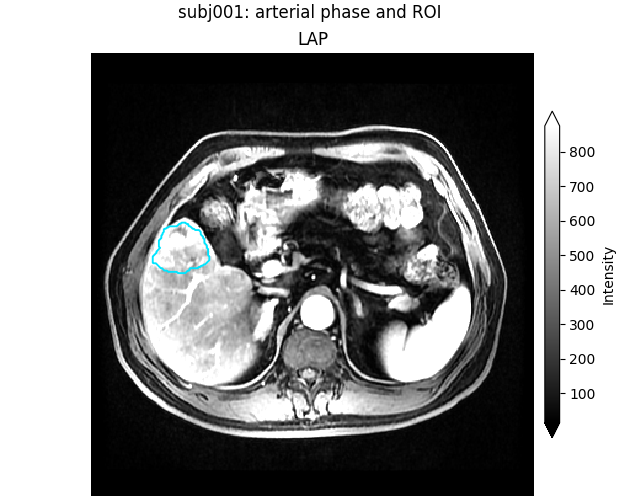
Four subjects define the habitats; the fifth plays a new patient later. The downloaded pack is cached after the first run. sphinx_gallery_thumbnail_number = 4

from pathlib import Path

import matplotlib.pyplot as plt
import numpy as np

from habit.contracts import HabitatModel, cohort_from_directory
from habit.datasets import fetch_demo
from habit.kernels import habitat_ith_dispersion, ith_score, spatial_interaction_matrix
from habit.recipes import Study, two_step_habitat
from habit.spec import HabitatSpec, Spec, Stage
from habit.viz import (
    plot_cluster_validation_from_report,
    plot_habitat_graph_slice,
    plot_habitat_overlay,
    plot_habitat_volume_fractions,
    plot_intensity_slice,
    plot_ith_summary,
    plot_msi_matrix,
    plot_partition_triptych,
)

# Change DATA / MODALITIES / ROI to your preprocessed layout.
DATA = fetch_demo()
MODALITIES = ("pre_contrast", "LAP", "PVP", "delay_3min")
ROI = "LAP"
cohort = cohort_from_directory(DATA, modalities=MODALITIES, roi=ROI)
train, new_patient = cohort[:4], cohort[4:]
print(cohort)

subject = train[0]
Path("out").mkdir(exist_ok=True)
fig = plot_intensity_slice(
    subject.image("LAP"),
    roi_mask=subject.mask(ROI),
    roi_contour=True,
    image_label="LAP",
    title=f"{subject.subject_id}: arterial phase and ROI",
)
fig.savefig("out/quickstart_input.png", dpi=150, bbox_inches="tight")
plt.show()

HABIT demo data (cached)
DATA (preprocessed root): C:\Users\dongm\.habit_data\demo-data-v1\preprocessed

On-disk inventory of this folder:
  subjects (5): subj001, subj002, subj003, subj004, subj005
  image series: LAP, PVP, delay_3min, pre_contrast
  mask keys:    LAP, PVP, delay_3min, pre_contrast
  example image: images/subj001/delay_3min/WATER__BH_Ax_LAVA_Flex_3min_Series0012.nrrd
  example mask:  masks/subj001/delay_3min/WATER__BH_Ax_LAVA_Flex_10min_Series0017_mask.nrrd

Your own data must use the same folder tree (change IDs / series names):

  DATA/
    images/<subject_id>/<modality>/<one image file>
    masks/<subject_id>/<roi>/<one mask file>

Then load it with the same call the demos use:

  cohort = cohort_from_directory(DATA, modalities=("LAP",), roi="LAP")

Swap DATA / modalities / roi to match your tree. Mask key is often the
same as one image series (here LAP).
Cohort(5 subjects [subj001, subj002, subj003, subj004, subj005])
F:\work\habit_project\habit\viz\intensity.py:616: UserWarning: Display geometry conflict: image/anatomy direction does not match mask/label direction. Using the mask/label direction so coronal/sagittal superior-up follows the labelled anatomy. Pass direction= to override.
  resolved_direction, resolved_spacing = resolve_display_geometry(

Build the analysis step by step

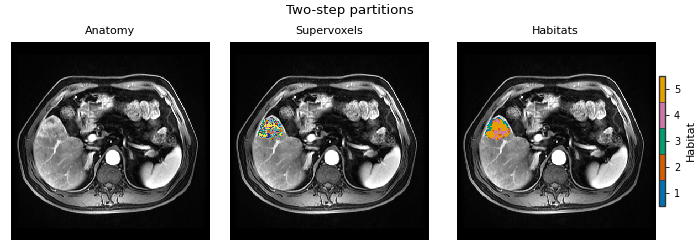
A habitat analysis is a list of stages. This is the two-step design: each tumour is split into 30 supervoxels (partition), the supervoxels of all subjects are put together (pool) and clustered once (fit), so habitat 2 means the same enhancement pattern in every patient. Drop pool and every subject is clustered on its own (one-step); drop partition and voxels are clustered directly (direct pooling). The fitter tries 2 to 10 habitats and keeps the elbow.

spec = HabitatSpec(
    name="quickstart_two_step",
    stages=(
        # extract: one intensity column per DCE phase, inside the ROI.
        Stage("extract", Spec("raw", {"modalities": list(MODALITIES), "roi": ROI})),
        # partition: 30 supervoxels per tumour; these rows are clustered.
        Stage("partition", Spec("kmeans", {"n_supervoxels": 30})),
        # pool: one matrix for every training subject, then one fit.
        Stage("pool", Spec("pool")),
        # fit: search 2..10 habitats and keep the elbow. n_init=10 restarts.
        Stage("fit", Spec("kmeans", {"min_habitats": 2, "max_habitats": 10, "validation": "elbow", "n_init": 10})),
        # assign: nearest centroid writes the shared habitat ids.
        Stage("assign", Spec("nearest_centroid")),
        # quantify: one row per subject. Spec name is the feature family.
        Stage("volume", Spec("volume")),
        Stage("msi", Spec("msi")),
        Stage("ith", Spec("ith_score")),
        Stage("graph", Spec("graph", {"include_extended_metrics": False})),
    ),
    # Seeds partition and fit. It is not a RunPolicy setting.
    random_seed=0,
)
# Study runs the spec: fit_predict learns the habitats on the four training
# subjects and labels those same subjects in one call.
result = Study(spec).fit_predict(train)
print(result.habitat_model.summary())

Cohort.map[_ComputeUnits]:   0%|          | 0/4 [00:00<?, ?it/s]
Cohort.map[_ComputeUnits]:  25%|██▌       | 1/4 [00:05<00:17,  5.74s/it]
Cohort.map[_ComputeUnits]:  50%|█████     | 2/4 [00:07<00:07,  3.59s/it]
Cohort.map[_ComputeUnits]:  75%|███████▌  | 3/4 [00:08<00:02,  2.83s/it]
Cohort.map[_ComputeUnits]: 100%|██████████| 4/4 [00:09<00:00,  2.46s/it]
Cohort.map[_ComputeUnits]: 100%|██████████| 4/4 [00:09<00:00,  2.46s/it]

Cohort.map[_AssignPrecomputedUnits]:   0%|          | 0/4 [00:00<?, ?it/s]
Cohort.map[_AssignPrecomputedUnits]:  25%|██▌       | 1/4 [00:01<00:04,  1.41s/it]
Cohort.map[_AssignPrecomputedUnits]:  50%|█████     | 2/4 [00:02<00:02,  1.10s/it]
Cohort.map[_AssignPrecomputedUnits]:  75%|███████▌  | 3/4 [00:02<00:00,  1.02it/s]
Cohort.map[_AssignPrecomputedUnits]: 100%|██████████| 4/4 [00:03<00:00,  1.09it/s]
Cohort.map[_AssignPrecomputedUnits]: 100%|██████████| 4/4 [00:03<00:00,  1.09it/s]
HabitatModel kmeans-b01ecfd00139f26e
  habitats           : 5
  features (4)    : pre_contrast, LAP, PVP, delay_3min
  defining cohort    : n=4
  modalities         : pre_contrast, LAP, PVP, delay_3min
  cohort digest      : 81dc6515a9f2b393...
  produced by        : habitat_model_fitter.kmeans
  habit version      : 3.0.0
  random seed        : 0
  preprocessing state: inertia, selection_report, validation

two_step_habitat(modalities=..., roi=..., n_supervoxels=30, habitat_features=[...], random_seed=0) is a shortcut for the same spec; one_step_habitat and direct_pooling_habitat do the same for the other designs. Both give the same habitat maps:

shortcut = two_step_habitat(modalities=MODALITIES, roi=ROI, n_supervoxels=30, random_seed=0).fit_predict(train)
same = all(np.array_equal(a.label_array, b.label_array) for a, b in zip(result.habitat_maps, shortcut.habitat_maps))
print("stages == shortcut:", same)

Cohort.map[_ComputeUnits]:   0%|          | 0/4 [00:00<?, ?it/s]
Cohort.map[_ComputeUnits]:  25%|██▌       | 1/4 [00:02<00:06,  2.02s/it]
Cohort.map[_ComputeUnits]:  50%|█████     | 2/4 [00:03<00:03,  1.92s/it]
Cohort.map[_ComputeUnits]:  75%|███████▌  | 3/4 [00:05<00:01,  1.70s/it]
Cohort.map[_ComputeUnits]: 100%|██████████| 4/4 [00:06<00:00,  1.61s/it]
Cohort.map[_ComputeUnits]: 100%|██████████| 4/4 [00:06<00:00,  1.61s/it]

Cohort.map[_AssignPrecomputedUnits]:   0%|          | 0/4 [00:00<?, ?it/s]
Cohort.map[_AssignPrecomputedUnits]:  25%|██▌       | 1/4 [00:00<00:00,  4.49it/s]
Cohort.map[_AssignPrecomputedUnits]:  50%|█████     | 2/4 [00:00<00:00,  4.61it/s]
Cohort.map[_AssignPrecomputedUnits]:  75%|███████▌  | 3/4 [00:00<00:00,  4.67it/s]
Cohort.map[_AssignPrecomputedUnits]: 100%|██████████| 4/4 [00:00<00:00,  4.71it/s]
Cohort.map[_AssignPrecomputedUnits]: 100%|██████████| 4/4 [00:00<00:00,  4.71it/s]
stages == shortcut: True

How many habitats, and why

The fitter scores every candidate count; the marked point is the one kept. The report travels inside the model, so the choice is auditable.

report = result.habitat_model.preprocessing_state["selection_report"]
fig = plot_cluster_validation_from_report(report)
fig.savefig("out/quickstart_elbow.png", dpi=150, bbox_inches="tight")
plt.show()

Habitat maps

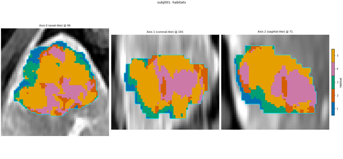
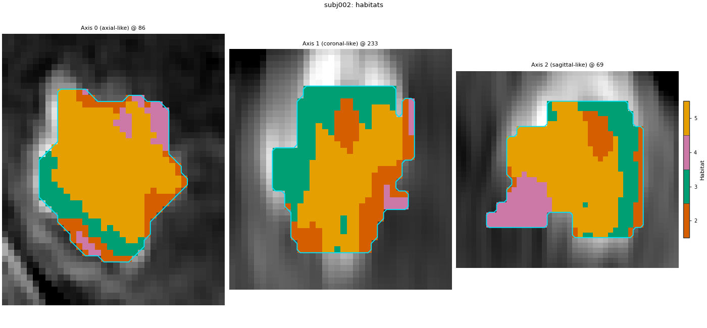
From supervoxels to habitats on one slice, then the habitat map of two patients. Same colour, same habitat, in both.

habitat_map = result.habitat_maps[0]
fig = plot_partition_triptych(subject.image("LAP"), result.units[0], habitat_map, axis=0)
fig.savefig("out/quickstart_triptych.png", dpi=150, bbox_inches="tight")
plt.show()

for other in (0, 1):
    fig = plot_habitat_overlay(
        train[other].image("LAP"),
        result.habitat_maps[other],
        title=f"{train[other].subject_id}: habitats",
        crop_to="labels",
    )
    fig.savefig(f"out/quickstart_habitats_{train[other].subject_id}.png", dpi=150, bbox_inches="tight")
    plt.show()

• 
• 
• 

F:\work\habit_project\habit\viz\habitat_core.py:1110: UserWarning: Display geometry conflict: image/anatomy direction does not match mask/label direction. Using the mask/label direction so coronal/sagittal superior-up follows the labelled anatomy. Pass direction= to override.
  resolved_direction, resolved_spacing = resolve_display_geometry(
F:\work\habit_project\habit\viz\habitat_overlay.py:806: UserWarning: Display geometry conflict: image/anatomy direction does not match mask/label direction. Using the mask/label direction so coronal/sagittal superior-up follows the labelled anatomy. Pass direction= to override.
  resolved_direction, resolved_spacing = resolve_display_geometry(
F:\work\habit_project\habit\viz\habitat_overlay.py:806: UserWarning: Display geometry conflict: image/anatomy direction does not match mask/label direction. Using the mask/label direction so coronal/sagittal superior-up follows the labelled anatomy. Pass direction= to override.
  resolved_direction, resolved_spacing = resolve_display_geometry(

The feature table

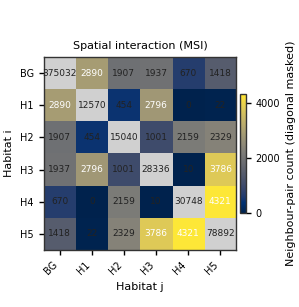
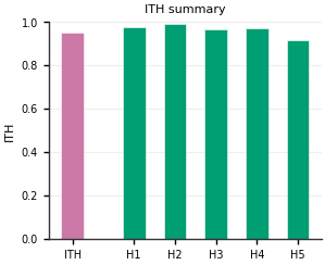
One row per subject, ready for statistics: volume fractions, the MSI (how habitats touch each other), the ITH score (how fragmented the tumour is) and graph topology. A few of the columns:

table = result.features.frame.set_index("subject")
print(table.shape[1], "columns")
columns = [c for c in table.columns if c.endswith("_volume_fraction")] + ["ith_score", "contrast", "graph_num_nodes_total"]
print(table[columns].round(3).to_string())

663 columns
         habitat_1_volume_fraction  habitat_2_volume_fraction  habitat_3_volume_fraction  habitat_4_volume_fraction  habitat_5_volume_fraction  ith_score  contrast  graph_num_nodes_total
subject
subj001                      0.090                      0.110                      0.182                      0.182                      0.436      0.949     1.424                  498.0
subj002                      0.000                      0.171                      0.196                      0.117                      0.516      0.850     2.295                  125.0
subj003                      0.000                      0.424                      0.000                      0.576                      0.000      0.796     1.639                   47.0
subj004                      0.178                      0.169                      0.550                      0.000                      0.104      0.862     1.461                  105.0

What those numbers look like for one subject

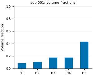
Volume fractions come straight from the table. MSI and ITH are drawn from the same label map with the kernels the table uses.

labels = habitat_map.label_array
fractions = {hid: float(table.loc[subject.subject_id, f"habitat_{hid}_volume_fraction"]) for hid in habitat_map.habitat_ids}
fig = plot_habitat_volume_fractions(fractions, title=f"{subject.subject_id}: volume fractions")
fig.savefig("out/quickstart_volume_fractions.png", dpi=150, bbox_inches="tight")
plt.show()

n_classes = max(habitat_map.habitat_ids) + 1
fig = plot_msi_matrix(spatial_interaction_matrix(labels, n_classes=n_classes), habitat_ids=habitat_map.habitat_ids)
fig.savefig("out/quickstart_msi.png", dpi=150, bbox_inches="tight")
plt.show()

fig = plot_ith_summary(float(ith_score(labels)), dispersion=habitat_ith_dispersion(labels))
fig.savefig("out/quickstart_ith.png", dpi=150, bbox_inches="tight")
plt.show()

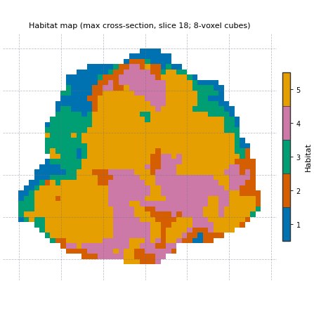
# The graph features cut the tumour into 8-voxel cubes (the grid); each
# cube is a node coloured by its habitat, and touching cubes share an edge.
fig = plot_habitat_graph_slice(labels, block_size=8)
fig.savefig("out/quickstart_graph.png", dpi=150, bbox_inches="tight")
plt.show()

• 
• 
• 
• 

Reuse the model on a new patient

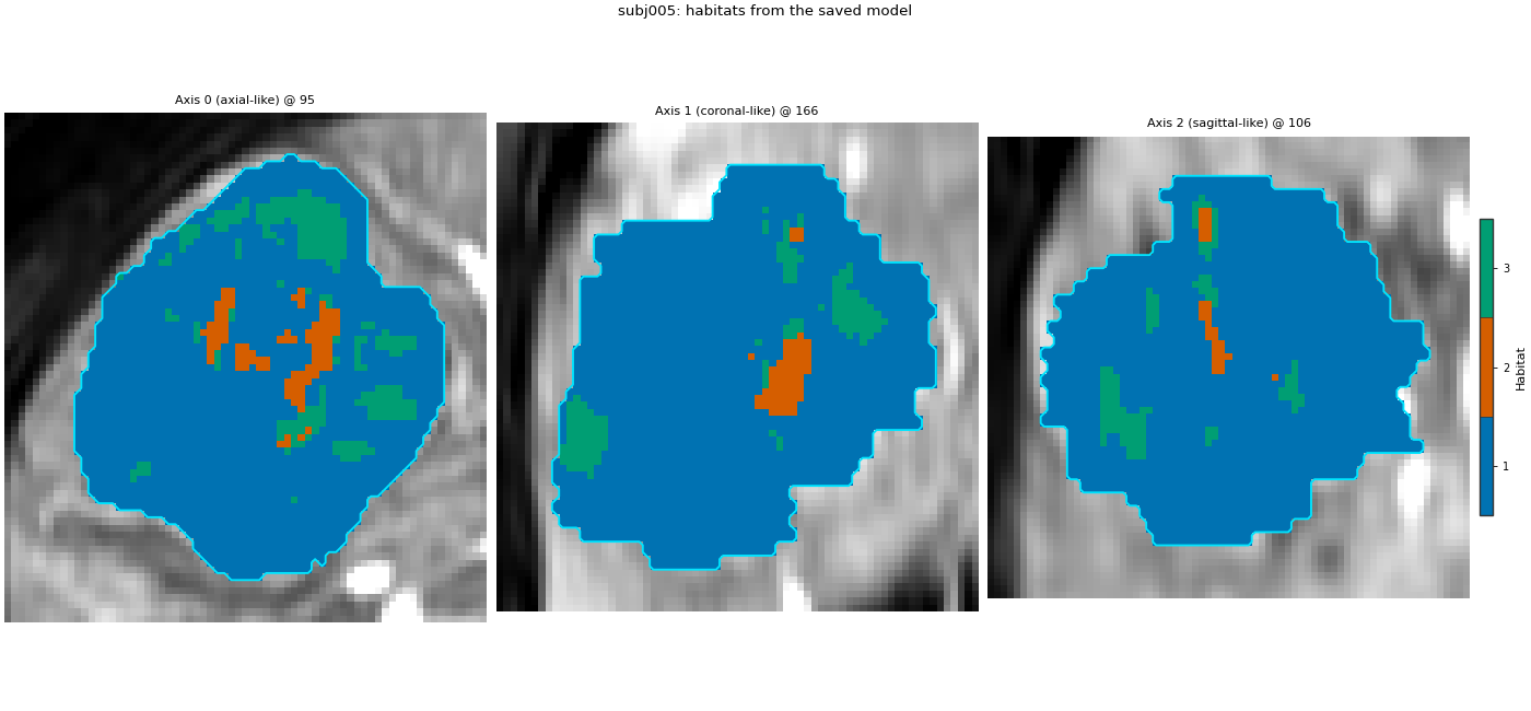
The .habitatmodel file is the habitat definition: load it anywhere and the new patient gets the same habitat names. Nothing is refitted. save writes the model archive and result tables under out/quickstart, plus the habitat maps because write_maps=True.

result.save("out/quickstart", write_maps=True)
model = HabitatModel.load("out/quickstart/habitat_model.habitatmodel")
# predict labels the held-out fifth subject with the saved centroids.
prediction = Study.from_model(model).predict(new_patient)
fig = plot_habitat_overlay(
    new_patient[0].image("LAP"),
    prediction.habitat_maps[0],
    title=f"{new_patient[0].subject_id}: habitats from the saved model",
    crop_to="labels",
)
fig.savefig("out/quickstart_new_patient.png", dpi=150, bbox_inches="tight")
plt.show()

Cohort.map[_LabelAndDescribe]:   0%|          | 0/1 [00:00<?, ?it/s]
Cohort.map[_LabelAndDescribe]: 100%|██████████| 1/1 [00:04<00:00,  4.63s/it]
Cohort.map[_LabelAndDescribe]: 100%|██████████| 1/1 [00:04<00:00,  4.63s/it]
F:\work\habit_project\habit\viz\habitat_overlay.py:806: UserWarning: Display geometry conflict: image/anatomy direction does not match mask/label direction. Using the mask/label direction so coronal/sagittal superior-up follows the labelled anatomy. Pass direction= to override.
  resolved_direction, resolved_spacing = resolve_display_geometry(

Where to go next

• The same analysis from a YAML file: Quickstart: YAML, and from the shell with habit get-habitat --config config/habitat/config_habitat_quickstart_v1.yaml (Quickstart: run the demo (YAML + CLI)). Both fit the same four subjects and give the same habitat maps as this page.

• The same stages, then each one opened up: A complete habitat analysis.

• Interactive 3-D view (pip install "habitat-analysis[view]"):

  from habit.viz import view_habitat_napari
  view_habitat_napari(subject.image("LAP"), habitat_map)