Matching habitat labels across subjects

Background. In a one_step study each patient is clustered on its own, so habitat ids are not comparable between patients until they are matched onto shared prototypes.

Purpose. This is the practical page: one call gives every demo subject shared habitat ids, and you see the renames, a centroid plot before and after naming, and the optional settings (max_distance, frozen prototypes, other distances).

When to use. After per-subject (one_step) fits. Skip it for two-step or direct-pooling studies, which already share one id space.

Key terms.

• one_step – habitats are clustered separately inside each subject, with no shared cohort model.

• prototype – a shared reference habitat (one feature row); see Prototype matching step by step.

• label switching – see Why habitat ids must be matched.

With one_step habitats every subject is clustered on its own, so habitat 1 of one patient need not be habitat 1 of another, and patients may even have different habitat counts. align_habitat_maps_to_prototypes() gives every subject one shared set of names:

• K shared prototypes, K = the largest habitat count in the cohort;

• each subject is matched one-to-one onto the prototypes, so no habitat is merged, dropped, or renamed twice;

• prototypes move to the mean of their matched habitats, and the two steps repeat until nothing changes. No reference subject is chosen.

A habitat is described by the fitted clustering centroids by default (models=); per-habitat means of a voxel feature field (features=) or your own matrices (centroids=) also work. Method, worked numbers, and literature: Matching habitat labels across fits and subjects. Step-by-step pages (overlap cases, the prototype loop, distances, frozen prototypes, effect on cohort tables): 6. Matching Habitat Labels. A shared cohort model (two-step, direct pooling) already uses one id space and does not need this step.

One-step habitats on comparable features

Relative enhancement is a ratio to the unenhanced phase, so its values can be compared across patients; raw MRI signal cannot. Each subject picks its own habitat count (silhouette over 2..5), as one_step with n_habitats="auto" does. sphinx_gallery_thumbnail_number = 1

from pathlib import Path

import matplotlib.pyplot as plt
import numpy as np

from habit.contracts import Cohort, cohort_from_directory
from habit.datasets import fetch_demo
from habit.habitat_model import KMeansHabitatModelFitter
from habit.pipeline import voxel_units
from habit.precision import align_habitat_maps_to_prototypes
from habit.voxel_features import ExpressionVoxelFeatures

# Change DATA / MODALITIES / ROI and the expressions to your own layout.
DATA = fetch_demo()
MODALITIES = ("pre_contrast", "LAP", "PVP")
ROI = "LAP"
cohort = cohort_from_directory(DATA, modalities=MODALITIES, roi=ROI)
extractor = ExpressionVoxelFeatures(
    features={
        "rel_enh_lap": "(LAP - pre_contrast) / (pre_contrast + eps)",
        "rel_enh_pvp": "(PVP - pre_contrast) / (pre_contrast + eps)",
    },
    roi=ROI,
)

maps, models, fields = [], [], []
for subject in cohort:
    field = extractor(subject)
    units = voxel_units(field)
    # Per-subject k-means; silhouette picks k in 2..5 for this subject alone.
    fitter = KMeansHabitatModelFitter(
        min_habitats=2, max_habitats=5, validation="silhouette", n_init=3
    )
    fitter.set_random_state(0)
    model = fitter.fit([units], cohort=Cohort([subject], name=subject.subject_id))
    maps.append(model.assigner()(units))
    models.append(model)
    fields.append(field)
    print(f"{subject.subject_id}: {model.n_habitats} habitats")

HABIT demo data (cached)
DATA (preprocessed root): C:\Users\dongm\.habit_data\demo-data-v1\preprocessed

On-disk inventory of this folder:
  subjects (5): subj001, subj002, subj003, subj004, subj005
  image series: LAP, PVP, delay_3min, pre_contrast
  mask keys:    LAP, PVP, delay_3min, pre_contrast
  example image: images/subj001/delay_3min/WATER__BH_Ax_LAVA_Flex_3min_Series0012.nrrd
  example mask:  masks/subj001/delay_3min/WATER__BH_Ax_LAVA_Flex_10min_Series0017_mask.nrrd

Your own data must use the same folder tree (change IDs / series names):

  DATA/
    images/<subject_id>/<modality>/<one image file>
    masks/<subject_id>/<roi>/<one mask file>

Then load it with the same call the demos use:

  cohort = cohort_from_directory(DATA, modalities=("LAP",), roi="LAP")

Swap DATA / modalities / roi to match your tree. Mask key is often the
same as one image series (here LAP).
subj001: 3 habitats
subj002: 2 habitats
subj003: 2 habitats
subj004: 2 habitats
subj005: 2 habitats

Name every subject against shared prototypes

models= reads each fitted HabitatModel.centroids: the habitats are named by the same features that defined them.

matched = align_habitat_maps_to_prototypes(maps, models=models)
print(f"K = {matched.prototypes.shape[0]} prototypes, features {matched.feature_names}")
print(matched.prototypes.round(3))
print(matched.assignments)
print(
    f"converged={matched.converged} after {matched.n_iter} rounds; "
    f"objective={matched.objective:.4f}"
)

K = 3 prototypes, features ('rel_enh_lap', 'rel_enh_pvp')
[[0.743 0.875]
 [1.579 1.321]
 [2.348 2.522]]
   subject_id  habitat_id  prototype_id  distance
0     subj001           1             3  1.169320
1     subj001           2             1  0.243208
2     subj001           3             2  0.252343
3     subj002           1             2  0.622436
4     subj002           2             1  0.217232
5     subj003           1             2  0.977614
6     subj003           2             1  0.479651
7     subj004           1             1  0.110715
8     subj004           2             2  0.229047
9     subj005           1             3  1.169320
10    subj005           2             2  0.828704
converged=True after 2 rounds; objective=5.2293

Every subject keeps its habitat count; ids now share one meaning.

for subject_id, rows in matched.assignments.groupby("subject_id"):
    renames = ", ".join(
        f"{old}->{new}" for old, new in zip(rows.habitat_id, rows.prototype_id)
    )
    print(f"{subject_id}: {renames}")

subj001: 1->3, 2->1, 3->2
subj002: 1->2, 2->1
subj003: 1->2, 2->1
subj004: 1->1, 2->2
subj005: 1->3, 2->2

Same call with voxel features instead of fitted centroids

features= averages each habitat’s voxels of the given field. Here it is the clustering field itself, so the prototypes agree with the models= result up to k-means convergence.

from_features = align_habitat_maps_to_prototypes(maps, features=fields)
gap = float(np.max(np.abs(from_features.prototypes - matched.prototypes)))
print(f"largest prototype difference, features= vs models=: {gap:.2e}")

largest prototype difference, features= vs models=: 1.18e-03

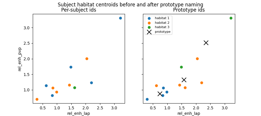
Centroids before and after naming

Path("out").mkdir(exist_ok=True)
table = matched.assignments
points = np.vstack([np.asarray(m.centroids) for m in models])
colours = plt.get_cmap("tab10")
fig, axes = plt.subplots(1, 2, figsize=(9, 4), sharex=True, sharey=True)
for axis, column, title in (
    (axes[0], "habitat_id", "Per-subject ids"),
    (axes[1], "prototype_id", "Prototype ids"),
):
    ids = table[column].to_numpy()
    for habitat_id in sorted(set(int(v) for v in ids)):
        chosen = ids == habitat_id
        axis.scatter(
            points[chosen, 0],
            points[chosen, 1],
            color=colours(habitat_id - 1),
            label=f"habitat {habitat_id}",
        )
    axis.set_title(title)
    axis.set_xlabel(matched.feature_names[0])
axes[1].scatter(
    matched.prototypes[:, 0],
    matched.prototypes[:, 1],
    marker="x",
    s=120,
    color="black",
    label="prototype",
)
axes[0].set_ylabel(matched.feature_names[1])
axes[1].legend(loc="best", fontsize=8)
fig.suptitle("Subject habitat centroids before and after prototype naming")
fig.savefig("out/match_labels_prototypes.png", dpi=150, bbox_inches="tight")
plt.show()

Optional: refuse far matches

By default every habitat is named. max_distance (feature units) leaves a habitat unnamed when every free prototype is farther than that; its prototype_id is NA and its voxels get a subject-local id above K. Keep it off when the aligned maps feed a cohort feature table.

partial = align_habitat_maps_to_prototypes(maps, models=models, max_distance=1.0)
print(partial.assignments[partial.assignments.prototype_id.isna()])

  subject_id  habitat_id  prototype_id  distance
6    subj003           2          <NA>       NaN
9    subj005           1          <NA>       NaN

Name new subjects with frozen prototypes

A validation cohort must be named with the training definition, not refitted together with it. Fit prototypes on the first three subjects, then pass that result as prototypes=: the last two subjects are assigned to the stored prototypes and share the training model_id.

trained = align_habitat_maps_to_prototypes(maps[:3], models=models[:3])
named = align_habitat_maps_to_prototypes(maps[3:], models=models[3:], prototypes=trained)
print(f"trained K = {trained.prototypes.shape[0]}, model_id {trained.model_id}")
print(f"new maps model_id {named.habitat_maps[0].model_id}")
print(named.assignments)

trained K = 3, model_id prototype-25d5b941c0235fd6
new maps model_id prototype-25d5b941c0235fd6
  subject_id  habitat_id  prototype_id  distance
0    subj004           1             1  0.147620
1    subj004           2             2  0.051461
2    subj005           1             3  2.338639
3    subj005           2             2  1.029463

Other distances

metric="manhattan" (median prototypes) is less pulled by one outlying habitat. "cosine" / "correlation" compare only the direction / shape of the feature vector and ignore its level, which for two enhancement features would merge weak and strong habitats; keep the default "sqeuclidean" for such features.

robust = align_habitat_maps_to_prototypes(maps, models=models, metric="manhattan")
print(robust.prototypes.round(3))

[[0.847 0.872]
 [1.616 1.151]
 [2.348 2.522]]