Multiregional spatial interaction (MSI)

Background. Two tumours can have the same habitat fractions but a different spatial arrangement: habitats mixed together, or kept apart. MSI measures that arrangement by counting which habitats touch which.

Purpose. You get the MSI matrix as a table and heatmap, plus a dictionary of scalar MSI features (one value per name) ready to use as columns in a statistics or model table.

Key terms.

• MSI (multiregional spatial interaction, Wu et al. 2018) – counts how often voxels of each habitat touch voxels of each other habitat (face neighbours), describing how habitats are arranged in space.

• MSI matrix – entry [i, j] is the number of face-neighbour voxel pairs labelled i and j; row/column 0 is background, so it records how much of each habitat lies on the tumour border.

• MSI scalars – firstorder_* are the matrix entries (raw and normalised); contrast / homogeneity / correlation / energy are texture-style summaries of the normalised matrix.

Atomic MSI from a habitat label map (Wu et al., Radiology 2018): spatial_interaction_matrix() and msi_features_from_matrix().

Build a habitat map, then compute the MSI matrix and scalar summaries. sphinx_gallery_thumbnail_number = 1

from pathlib import Path

import matplotlib.pyplot as plt
import pandas as pd

from habit.contracts import cohort_from_directory
from habit.datasets import fetch_demo
from habit.kernels import msi_features_from_matrix, spatial_interaction_matrix
from habit.recipes import one_step_habitat
from habit.viz import plot_msi_matrix

DATA = fetch_demo()
MODALITIES = ("LAP",)
ROI = "LAP"
cohort = cohort_from_directory(DATA, modalities=MODALITIES, roi=ROI)[:1]
result = one_step_habitat(
    modalities=MODALITIES, n_habitats=3, random_seed=0, roi=ROI
).fit_predict(cohort)
habitat_map = result.habitat_maps[0]
labels = habitat_map.label_array
ids = tuple(sorted({int(v) for v in labels.ravel() if int(v) != 0}))
# Matrix size includes background (class 0), hence the + 1.
n_classes = int(max(ids)) + 1

HABIT demo data (cached)
DATA (preprocessed root): C:\Users\dongm\.habit_data\demo-data-v1\preprocessed

On-disk inventory of this folder:
  subjects (5): subj001, subj002, subj003, subj004, subj005
  image series: LAP, PVP, delay_3min, pre_contrast
  mask keys:    LAP, PVP, delay_3min, pre_contrast
  example image: images/subj001/delay_3min/WATER__BH_Ax_LAVA_Flex_3min_Series0012.nrrd
  example mask:  masks/subj001/delay_3min/WATER__BH_Ax_LAVA_Flex_10min_Series0017_mask.nrrd

Your own data must use the same folder tree (change IDs / series names):

  DATA/
    images/<subject_id>/<modality>/<one image file>
    masks/<subject_id>/<roi>/<one mask file>

Then load it with the same call the demos use:

  cohort = cohort_from_directory(DATA, modalities=("LAP",), roi="LAP")

Swap DATA / modalities / roi to match your tree. Mask key is often the
same as one image series (here LAP).

Cohort.map[_DefineAndLabelWithinSubject]:   0%|          | 0/1 [00:00<?, ?it/s]
Cohort.map[_DefineAndLabelWithinSubject]: 100%|██████████| 1/1 [00:01<00:00,  1.29s/it]
Cohort.map[_DefineAndLabelWithinSubject]: 100%|██████████| 1/1 [00:01<00:00,  1.29s/it]

MSI matrix (background row/column 0) and derived scalar features.

matrix = spatial_interaction_matrix(labels, n_classes=n_classes)
msi_table = pd.DataFrame(
    matrix,
    index=["BG"] + [f"H{i}" for i in range(1, n_classes)],
    columns=["BG"] + [f"H{i}" for i in range(1, n_classes)],
)
print("MSI matrix:")
print(msi_table.round(4).head())
msi_table.head()

# Flatten the matrix into named scalars (same keys as HABIT v0.1 MSI output).
features = msi_features_from_matrix(matrix)
print("MSI scalars:", {k: round(v, 4) for k, v in features.items()})

Path("out").mkdir(exist_ok=True)
fig_msi = plot_msi_matrix(matrix, habitat_ids=tuple(range(1, n_classes)))
fig_msi.savefig("out/msi_matrix_heatmap.png", dpi=150, bbox_inches="tight")
plt.show()

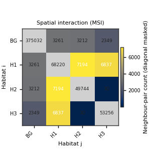
MSI matrix:
        BG     H1     H2     H3
BG  375032   3261   3212   2349
H1    3261  68220   7194   6837
H2    3212   7194  49744     30
H3    2349   6837     30  53256
MSI scalars: {'firstorder_0_and_1': 3261.0, 'firstorder_0_and_2': 3212.0, 'firstorder_0_and_3': 2349.0, 'firstorder_1_and_2': 7194.0, 'firstorder_1_and_3': 6837.0, 'firstorder_2_and_3': 30.0, 'firstorder_1_and_1': 68220.0, 'firstorder_2_and_2': 49744.0, 'firstorder_3_and_3': 53256.0, 'firstorder_normalized_0_and_1': 0.0168, 'firstorder_normalized_0_and_2': 0.0165, 'firstorder_normalized_0_and_3': 0.0121, 'firstorder_normalized_1_and_2': 0.0371, 'firstorder_normalized_1_and_3': 0.0352, 'firstorder_normalized_2_and_3': 0.0002, 'firstorder_normalized_1_and_1': 0.3515, 'firstorder_normalized_2_and_2': 0.2563, 'firstorder_normalized_3_and_3': 0.2744, 'contrast': 0.74, 'homogeneity': 2.8914, 'correlation': 0.0115, 'energy': 4.0042}