Running the same study on each backend

Background. Once a study is declared, HABIT still has to run it on every subject. This page is about that scheduling layer. Switching the backend or RunPolicy changes speed and how failures are handled; it does not change the science, so the habitat labels must come out identical.

Purpose. You will run one study serially and with process workers and confirm the labels match, see why serial can win on a tiny cohort, keep a run going when one subject fails, resume from checkpoints, and build policies for GPU worker caps and per-subject timeouts.

When to use. Stay serial for a handful of subjects or while debugging one case. Switch to process workers when there are many subjects and each one is expensive.

Key terms.

• backend – what schedules the subjects: serial (one after another in this Python process) or a pool of worker processes.

• RunPolicy – the settings object for a run: backend, number of workers, failure handling, timeouts, checkpoint and resume options.

• spawn – how Windows starts a worker: a fresh Python interpreter that re-imports HABIT, which costs seconds per worker.

• checkpoint – finished subject results saved on disk so an interrupted run resumes without recomputing them.

• supervoxel / pool / fit / assign – the study stages; see A complete habitat analysis.

The study is the two-step list from A complete habitat analysis, with the habitat count fixed at 3 so this page can refit it on every backend. Only backend= / RunPolicy settings change. Habitat labels must match.

Where the work runs	What to pass
This process, one subject at a time	SerialBackend()
CPU, several subjects at once	RunPolicy(backend="process")
A fresh process per subject	parallel_mode="isolated"
One worker per GPU	cap_workers_to_gpu_pool=True

backend is only "serial" or "process". Isolated mode and the GPU cap are settings of the process backend, not extra backend names. On one GPU only worker 0 gets the card unless HABIT_GPU_OVERSUBSCRIBE=wrap.

On Windows a process pool must start under if __name__ == "__main__": (a spawned worker re-imports this file). Each backend cell below is written that way so it can be copied as is.

Load the cohort and declare the study

Same stages as the complete analysis, except fit uses n_habitats=3 instead of an elbow search. sphinx_gallery_thumbnail_number = 1

import dataclasses
import tempfile
import time
from pathlib import Path

import matplotlib.pyplot as plt
import numpy as np

from habit.contracts import Cohort, cohort_from_directory
from habit.datasets import fetch_demo
from habit.execution import CheckpointStore, SerialBackend, backend_from_policy
from habit.recipes import Study
from habit.spec import HabitatSpec, RunPolicy, Spec, Stage
from habit.viz import plot_habitat_overlay

# Change DATA / MODALITIES / ROI to your preprocessed layout.
# The guard keeps a spawned worker from loading the cohort again.
if __name__ == "__main__":
    DATA = fetch_demo()
    MODALITIES = ("pre_contrast", "LAP", "PVP", "delay_3min")
    ROI = "LAP"
    cohort = cohort_from_directory(DATA, modalities=MODALITIES, roi=ROI)[:2]
    spec = HabitatSpec(
        name="parallel_backends",
        stages=(
            # extract: one intensity column per DCE phase, inside the ROI.
            Stage("extract", Spec("raw", {"modalities": list(MODALITIES), "roi": ROI})),
            # partition: 30 supervoxels per subject; these rows are clustered.
            Stage("partition", Spec("kmeans", {"n_supervoxels": 30})),
            # pool: one matrix for the whole training cohort.
            Stage("pool", Spec("pool")),
            # fit: fixed count so serial and process runs are the same model.
            Stage("fit", Spec("kmeans", {"n_habitats": 3, "n_init": 10})),
            # assign: nearest centroid writes the habitat ids.
            Stage("assign", Spec("nearest_centroid")),
            # quantify: volume fractions, so the result still has a feature table.
            Stage("volume", Spec("volume")),
        ),
        random_seed=0,
    )
    study = Study(spec)
    print(f"Cohort: {list(cohort.subject_ids)}")

HABIT demo data (cached)
DATA (preprocessed root): C:\Users\dongm\.habit_data\demo-data-v1\preprocessed

On-disk inventory of this folder:
  subjects (5): subj001, subj002, subj003, subj004, subj005
  image series: LAP, PVP, delay_3min, pre_contrast
  mask keys:    LAP, PVP, delay_3min, pre_contrast
  example image: images/subj001/delay_3min/WATER__BH_Ax_LAVA_Flex_3min_Series0012.nrrd
  example mask:  masks/subj001/delay_3min/WATER__BH_Ax_LAVA_Flex_10min_Series0017_mask.nrrd

Your own data must use the same folder tree (change IDs / series names):

  DATA/
    images/<subject_id>/<modality>/<one image file>
    masks/<subject_id>/<roi>/<one mask file>

Then load it with the same call the demos use:

  cohort = cohort_from_directory(DATA, modalities=("LAP",), roi="LAP")

Swap DATA / modalities / roi to match your tree. Mask key is often the
same as one image series (here LAP).
Cohort: ['subj001', 'subj002']

Serial backend

One subject after another, in this process. This is the reference the other backends must match.

if __name__ == "__main__":
    timings: dict[str, float] = {}
    start = time.perf_counter()
    serial = study.fit_predict(cohort, backend=SerialBackend())
    timings["serial"] = time.perf_counter() - start
    print(f"serial: {timings['serial']:.1f} s, backend SerialBackend")
    print(serial.features.frame)

Cohort.map[_ComputeUnits]:   0%|          | 0/2 [00:00<?, ?it/s]
Cohort.map[_ComputeUnits]:  50%|█████     | 1/2 [00:02<00:02,  2.10s/it]
Cohort.map[_ComputeUnits]: 100%|██████████| 2/2 [00:03<00:00,  1.77s/it]
Cohort.map[_ComputeUnits]: 100%|██████████| 2/2 [00:03<00:00,  1.78s/it]

Cohort.map[_AssignPrecomputedUnits]:   0%|          | 0/2 [00:00<?, ?it/s]
Cohort.map[_AssignPrecomputedUnits]:  50%|█████     | 1/2 [00:00<00:00,  3.26it/s]
Cohort.map[_AssignPrecomputedUnits]: 100%|██████████| 2/2 [00:00<00:00,  3.19it/s]
Cohort.map[_AssignPrecomputedUnits]: 100%|██████████| 2/2 [00:00<00:00,  3.19it/s]
serial: 4.2 s, backend SerialBackend
   subject  ...  habitat_3_volume_fraction
0  subj001  ...                   0.331844
1  subj002  ...                   0.569182

[2 rows x 7 columns]

Process backend, persistent workers

workers=2 asks for one process per subject. reuse_workers() keeps those interpreters warm after spawn; the first call still pays the Windows spawn + import cost.

if __name__ == "__main__":
    persistent = RunPolicy(workers=2, backend="process", parallel_mode="persistent")
    pool = backend_from_policy(persistent)
    print(type(pool).__name__, "workers", pool.workers, "mode", pool.policy.parallel_mode)
    with pool.reuse_workers():
        start = time.perf_counter()
        pooled = study.fit_predict(cohort, backend=pool)
        timings["process, persistent"] = time.perf_counter() - start
    print(f"process, persistent: {timings['process, persistent']:.1f} s")
    for left, right in zip(serial.habitat_maps, pooled.habitat_maps):
        print(
            f"{left.subject_id}: serial == persistent: "
            f"{np.array_equal(left.label_array, right.label_array)}"
        )

ProcessPoolBackend workers 2 mode persistent

Cohort.map[_ComputeUnits]:   0%|          | 0/2 [00:00<?, ?it/s]
Cohort.map[_ComputeUnits]:  50%|█████     | 1/2 [00:09<00:09,  9.83s/it]
Cohort.map[_ComputeUnits]: 100%|██████████| 2/2 [00:11<00:00,  5.58s/it]
Cohort.map[_ComputeUnits]: 100%|██████████| 2/2 [00:11<00:00,  5.58s/it]

Cohort.map[_AssignPrecomputedUnits]:   0%|          | 0/2 [00:00<?, ?it/s]
Cohort.map[_AssignPrecomputedUnits]:  50%|█████     | 1/2 [00:00<00:00,  3.22it/s]
Cohort.map[_AssignPrecomputedUnits]: 100%|██████████| 2/2 [00:00<00:00,  3.13it/s]
Cohort.map[_AssignPrecomputedUnits]: 100%|██████████| 2/2 [00:00<00:00,  3.12it/s]
process, persistent: 11.9 s
subj001: serial == persistent: True
subj002: serial == persistent: True

Process backend, one process per subject

parallel_mode="isolated" still uses backend="process". Each subject gets a new interpreter. Same labels, more start-up.

if __name__ == "__main__":
    isolated_policy = RunPolicy(workers=2, backend="process", parallel_mode="isolated")
    isolated = backend_from_policy(isolated_policy)
    print(type(isolated).__name__, "mode", isolated.policy.parallel_mode)
    start = time.perf_counter()
    isolated_result = study.fit_predict(cohort, backend=isolated)
    timings["process, isolated"] = time.perf_counter() - start
    print(f"process, isolated: {timings['process, isolated']:.1f} s")
    for left, right in zip(serial.habitat_maps, isolated_result.habitat_maps):
        print(
            f"{left.subject_id}: serial == isolated: "
            f"{np.array_equal(left.label_array, right.label_array)}"
        )

ProcessPoolBackend mode isolated

Cohort.map[_ComputeUnits]:   0%|          | 0/2 [00:00<?, ?it/s]
Cohort.map[_ComputeUnits]:  50%|█████     | 1/2 [00:08<00:08,  8.48s/it]
Cohort.map[_ComputeUnits]: 100%|██████████| 2/2 [00:09<00:00,  4.59s/it]
Cohort.map[_ComputeUnits]: 100%|██████████| 2/2 [00:09<00:00,  4.59s/it]

Cohort.map[_AssignPrecomputedUnits]:   0%|          | 0/2 [00:00<?, ?it/s]
Cohort.map[_AssignPrecomputedUnits]:  50%|█████     | 1/2 [00:00<00:00,  3.13it/s]
Cohort.map[_AssignPrecomputedUnits]: 100%|██████████| 2/2 [00:00<00:00,  3.15it/s]
Cohort.map[_AssignPrecomputedUnits]: 100%|██████████| 2/2 [00:00<00:00,  3.15it/s]
process, isolated: 9.9 s
subj001: serial == isolated: True
subj002: serial == isolated: True

Why serial can win on this tiny cohort

This demo uses only two subjects and a small fixed kmeans fit. On Windows the process backend uses spawn: each worker starts a new interpreter and imports HABIT. That start-up is often larger than the fit itself. Isolated mode pays spawn again for every subject. On a single GPU, cap_workers_to_gpu_pool=True leaves one worker, so “parallel” is not actually parallel.

The bar below is a cost demonstration, not a claim that serial is always faster. The scientific definition is unchanged: same HabitatSpec, same habitat labels. The timing gap is overhead. Process workers win when there are many subjects, each subject is expensive, and workers stays greater than 1. See the recorded multi-GPU table further down.

if __name__ == "__main__":
    for name, seconds in timings.items():
        print(f"{name}: {seconds:.1f} s")
    Path("out").mkdir(exist_ok=True)
    fig, ax = plt.subplots(figsize=(6.8, 2.8), constrained_layout=True)
    ax.barh(list(timings), list(timings.values()), color="#4C78A8")
    ax.invert_yaxis()
    ax.set_xlabel(f"wall-clock seconds ({len(cohort)} subjects)")
    ax.set_title("serial vs process pool vs isolated (tiny cohort)")
    fig.savefig("out/backends_timing.png", dpi=150, bbox_inches="tight")
    plt.show()

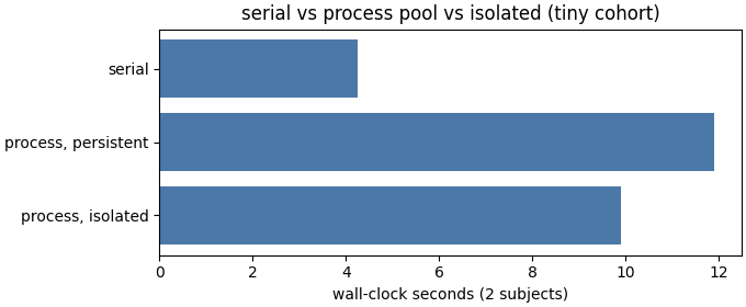
serial: 4.2 s
process, persistent: 11.9 s
process, isolated: 9.9 s

Cap workers to the GPU pool

Still backend="process". cap_workers_to_gpu_pool=True clamps workers to the visible cards, one worker per card. Building the policy does not launch a job. Set CUDA_VISIBLE_DEVICES before Python starts, for example 0,1,2,3,4, and leave HABIT_GPU_OVERSUBSCRIBE unset. The table is a recorded 5-GPU run (this machine is not asked to repeat it). Driver: scripts/run_multi_gpu_cohort_bench.py.

if __name__ == "__main__":
    gpu_policy = RunPolicy(
        workers=5,
        backend="process",
        parallel_mode="persistent",
        cap_workers_to_gpu_pool=True,
        on_subject_failure="fail_fast",
    )
    gpu_backend = backend_from_policy(gpu_policy)
    print(
        type(gpu_backend).__name__,
        "requested_workers=5",
        f"cap={gpu_backend.policy.cap_workers_to_gpu_pool}",
        f"workers_after_cap={gpu_backend.workers}",
    )

ProcessPoolBackend requested_workers=5 cap=True workers_after_cap=1

Scenario	Device	Workers	Pool	Wall (s)	Subjects/min	Speedup vs CPU serial
0 GPU	CUDA=-1 (CPU)	1	cold	263.49	3.64	1.00x
0 GPU	CUDA=-1 (CPU)	8	cold	49.16	19.53	5.36x
1 GPU	CUDA=0	1	warm	12.41	77.33	21.22x
5 GPUs	CUDA=0,1,2,3,4	5	cold	14.78	64.97	17.83x
5 GPUs	CUDA=0,1,2,3,4	5	warm	4.16	231.03	63.41x

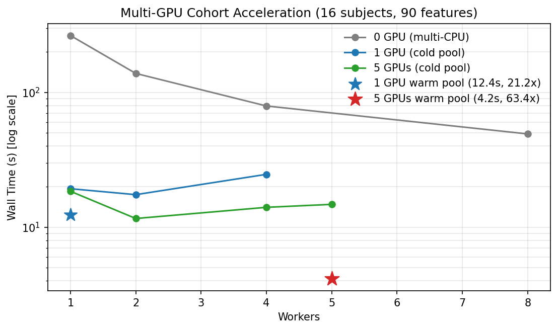
Recorded AutoDL result (16 subjects, 90 features, 2026-09-04). Stars are warm persistent pools. This page does not regenerate it.

Fault tolerance: continue vs fail_fast

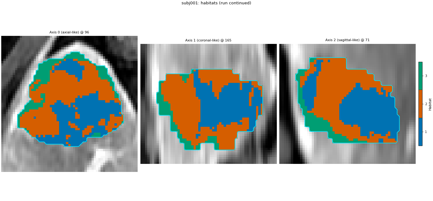
on_subject_failure is a RunPolicy / backend setting, not a separate backend. "continue" (the default) records the failed subject and still returns habitat maps for the subjects that worked. "fail_fast" raises at the first failure. Below, the fourth demo subject is copied without its portal-venous series, so extract cannot find PVP.

if __name__ == "__main__":
    sources = cohort_from_directory(DATA, modalities=MODALITIES, roi=ROI)[:4]
    broken = dataclasses.replace(
        sources[3],
        subject_id="subj004_no_PVP",
        images={name: ref for name, ref in sources[3].images.items() if name != "PVP"},
    )
    incomplete = Cohort(list(sources[:3]) + [broken], name="one_incomplete")
    continued = study.fit_predict(
        incomplete,
        backend=SerialBackend(on_subject_failure="continue"),
    )
    print("maps:", [one.subject_id for one in continued.habitat_maps])
    print("outcomes:", continued.manifest.subject_outcomes)
    try:
        study.fit_predict(
            incomplete,
            backend=SerialBackend(on_subject_failure="fail_fast"),
        )
    except KeyError as error:
        print("stopped:", error)

    fig = plot_habitat_overlay(
        incomplete[0].image(ROI),
        continued.habitat_maps[0],
        title=f"{incomplete[0].subject_id}: habitats (run continued)",
        crop_to="labels",
    )
    fig.savefig("out/backends_continued.png", dpi=150, bbox_inches="tight")
    plt.show()

Cohort.map[_ComputeUnits]:   0%|          | 0/4 [00:00<?, ?it/s]
Cohort.map[_ComputeUnits]:  25%|██▌       | 1/4 [00:02<00:06,  2.19s/it]
Cohort.map[_ComputeUnits]:  50%|█████     | 2/4 [00:03<00:03,  1.82s/it]
Cohort.map[_ComputeUnits]:  75%|███████▌  | 3/4 [00:04<00:01,  1.65s/it]
Cohort.map[_ComputeUnits]: 100%|██████████| 4/4 [00:05<00:00,  1.46s/it][habitat.units] subject subj004_no_PVP failed: KeyError: "Subject 'subj004_no_PVP' has no modality 'PVP'. Available: ['LAP', 'delay_3min', 'pre_contrast']."

Cohort.map[_ComputeUnits]: 100%|██████████| 4/4 [00:05<00:00,  1.46s/it]

Cohort.map[_AssignPrecomputedUnits]:   0%|          | 0/3 [00:00<?, ?it/s]
Cohort.map[_AssignPrecomputedUnits]:  33%|███▎      | 1/3 [00:00<00:00,  3.10it/s]
Cohort.map[_AssignPrecomputedUnits]:  67%|██████▋   | 2/3 [00:00<00:00,  3.12it/s]
Cohort.map[_AssignPrecomputedUnits]: 100%|██████████| 3/3 [00:00<00:00,  3.21it/s]
Cohort.map[_AssignPrecomputedUnits]: 100%|██████████| 3/3 [00:00<00:00,  3.21it/s]
maps: ['subj001', 'subj002', 'subj003']
outcomes: {'subj001': 'success', 'subj002': 'success', 'subj003': 'success', 'subj004_no_PVP': 'KeyError: "Subject \'subj004_no_PVP\' has no modality \'PVP\'. Available: [\'LAP\', \'delay_3min\', \'pre_contrast\']."'}

Cohort.map[_ComputeUnits]:   0%|          | 0/4 [00:00<?, ?it/s]
Cohort.map[_ComputeUnits]:  25%|██▌       | 1/4 [00:02<00:06,  2.03s/it]
Cohort.map[_ComputeUnits]:  50%|█████     | 2/4 [00:03<00:03,  1.73s/it]
Cohort.map[_ComputeUnits]:  75%|███████▌  | 3/4 [00:04<00:01,  1.57s/it]
Cohort.map[_ComputeUnits]:  75%|███████▌  | 3/4 [00:05<00:01,  1.86s/it]
stopped: "Subject 'subj004_no_PVP' has no modality 'PVP'. Available: ['LAP', 'delay_3min', 'pre_contrast']."
F:\work\habit_project\habit\viz\habitat_overlay.py:806: UserWarning: Display geometry conflict: image/anatomy direction does not match mask/label direction. Using the mask/label direction so coronal/sagittal superior-up follows the labelled anatomy. Pass direction= to override.
  resolved_direction, resolved_spacing = resolve_display_geometry(

Checkpoint resume

CheckpointStore writes finished subjects to disk. The first call runs the study and stores maps; the second call hits those checkpoints and finishes faster. Resume skips subjects already stored — it does not change habitat labels.

if __name__ == "__main__":
    store = CheckpointStore(Path(tempfile.mkdtemp(prefix="habit_ckpt_")))
    for attempt in ("first run", "rerun"):
        start = time.perf_counter()
        study.fit_predict(cohort, checkpoint=store)
        print(f"{attempt}: {time.perf_counter() - start:.1f} s")

Cohort.map[_ComputeUnits]:   0%|          | 0/2 [00:00<?, ?it/s]
Cohort.map[_ComputeUnits]:  50%|█████     | 1/2 [00:02<00:02,  2.25s/it]
Cohort.map[_ComputeUnits]: 100%|██████████| 2/2 [00:03<00:00,  1.90s/it]
Cohort.map[_ComputeUnits]: 100%|██████████| 2/2 [00:03<00:00,  1.90s/it]

Cohort.map[_AssignPrecomputedUnits]:   0%|          | 0/2 [00:00<?, ?it/s]
Cohort.map[_AssignPrecomputedUnits]:  50%|█████     | 1/2 [00:00<00:00,  1.99it/s]
Cohort.map[_AssignPrecomputedUnits]: 100%|██████████| 2/2 [00:00<00:00,  2.01it/s]
Cohort.map[_AssignPrecomputedUnits]: 100%|██████████| 2/2 [00:00<00:00,  2.01it/s]
first run: 4.9 s

Cohort.map[_ComputeUnits]:   0%|          | 0/2 [00:00<?, ?it/s]
Cohort.map[_ComputeUnits]:  50%|█████     | 1/2 [00:00<00:00, 26.82it/s]
Cohort.map[_ComputeUnits]: 100%|██████████| 2/2 [00:00<00:00, 27.03it/s]
Cohort.map[_ComputeUnits]: 100%|██████████| 2/2 [00:00<00:00, 27.03it/s]

Cohort.map[_AssignPrecomputedUnits]:   0%|          | 0/2 [00:00<?, ?it/s]
Cohort.map[_AssignPrecomputedUnits]:  50%|█████     | 1/2 [00:00<00:00, 13.91it/s]
Cohort.map[_AssignPrecomputedUnits]: 100%|██████████| 2/2 [00:00<00:00, 14.30it/s]
Cohort.map[_AssignPrecomputedUnits]: 100%|██████████| 2/2 [00:00<00:00, 14.19it/s]
rerun: 0.3 s

Per-subject timeout

subject_timeout_sec is a RunPolicy field. It is enforced only by the process backend (serial has no child to kill). The print below shows the policy object you would pass to backend_from_policy on a long cohort; this page does not wait for a real timeout.

if __name__ == "__main__":
    timeout = RunPolicy(
        workers=2,
        backend="process",
        on_subject_failure="continue",
        subject_timeout_sec=600,
    )
    print("timeout_sec", timeout.subject_timeout_sec, "on_failure", timeout.on_subject_failure)

timeout_sec 600 on_failure continue