Note
Go to the end to download the full example code.
Defining habitats in two steps
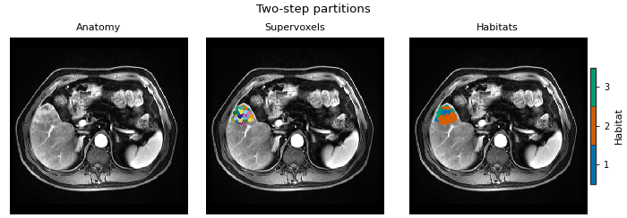
Background. The two-step design is the complete analysis used across this Guide: each tumour is first cut into supervoxels, then the supervoxels of all subjects are clustered together once, so habitat ids mean the same thing in every patient.
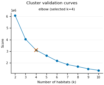
Purpose. You get one shared habitat model, a habitat map and a volume-fraction table per subject, a supervoxel / habitat triptych, and an elbow plot for choosing the habitat count.
When to use. You want habitats that are comparable across patients (e.g. volume fractions as cohort features) and whole-cohort voxel clustering would be slow or noisy.
Key terms.
supervoxel – a small patch of neighbouring voxels with similar features, clustered inside one subject first (
partition); see Partitioning a ROI into supervoxels.pool – stacks every training subject’s rows into one matrix so one model is fitted to the whole cohort.
SLIC – a supervoxel method that grows compact regions from a regular grid of seeds, trading intensity similarity against spatial distance.
elbow – see Quickstart: Python API.
Input: a cohort of at least two subjects. Output: one shared
HabitatModel and one
HabitatMap per subject. The design is the
stage list: partition then pool then fit.
SLIC is the partitioner here. Spec("kmeans", ...) in the
partition stage is the same study with a different partitioner, not
a second habitat definition to compare on this page. A fixed count of 3
draws the map; a 2-10 search draws the elbow on the same cohort.
two_step_habitat(...) is a shortcut that builds the same stage list.
Load the cohort
Change DATA / MODALITIES / ROI to your preprocessed layout.
sphinx_gallery_thumbnail_number = 2
from pathlib import Path

import matplotlib.pyplot as plt

from habit.contracts import cohort_from_directory
from habit.datasets import fetch_demo
from habit.recipes import Study
from habit.spec import HabitatSpec, Spec, Stage
from habit.viz import plot_cluster_validation_from_report, plot_partition_triptych

DATA = fetch_demo()
# Three DCE phases: unenhanced, arterial, and portal-venous.
MODALITIES = ("pre_contrast", "LAP", "PVP")
ROI = "LAP"
cohort = cohort_from_directory(DATA, modalities=MODALITIES, roi=ROI)[:2]
print(f"Cohort: {list(cohort.subject_ids)}")
HABIT demo data (cached)
DATA (preprocessed root): C:\Users\dongm\.habit_data\demo-data-v1\preprocessed

On-disk inventory of this folder:
  subjects (5): subj001, subj002, subj003, subj004, subj005
  image series: LAP, PVP, delay_3min, pre_contrast
  mask keys:    LAP, PVP, delay_3min, pre_contrast
  example image: images/subj001/delay_3min/WATER__BH_Ax_LAVA_Flex_3min_Series0012.nrrd
  example mask:  masks/subj001/delay_3min/WATER__BH_Ax_LAVA_Flex_10min_Series0017_mask.nrrd

Your own data must use the same folder tree (change IDs / series names):

  DATA/
    images/<subject_id>/<modality>/<one image file>
    masks/<subject_id>/<roi>/<one mask file>

Then load it with the same call the demos use:

  cohort = cohort_from_directory(DATA, modalities=("LAP",), roi="LAP")

Swap DATA / modalities / roi to match your tree. Mask key is often the
same as one image series (here LAP).
Cohort: ['subj001', 'subj002']
Supervoxels, clustering units, and habitats
fig = plot_partition_triptych(
    cohort[0].image(ROI),
    result.units[0],
    result.habitat_maps[0],
    axis=0,
)
Path("out").mkdir(exist_ok=True)
fig.savefig("out/two_step_triptych.png", dpi=150, bbox_inches="tight")
plt.show()
F:\work\habit_project\habit\viz\habitat_core.py:1110: UserWarning: Display geometry conflict: image/anatomy direction does not match mask/label direction. Using the mask/label direction so coronal/sagittal superior-up follows the labelled anatomy. Pass direction= to override.
  resolved_direction, resolved_spacing = resolve_display_geometry(
Elbow on the same stages, with fit searching 2-10 habitats. The
chosen count is the knee, not a second overlay. A saved model is
Applying a saved habitat model.
elbow_spec = HabitatSpec(
    name="two_step_slic_elbow",
    stages=first_stages + (
        Stage("fit", Spec("kmeans", {"min_habitats": 2, "max_habitats": 10, "validation": "elbow", "n_init": 10})),
        Stage("assign", Spec("nearest_centroid")),
    ),
    random_seed=0,
)
elbow = Study(elbow_spec).fit_predict(cohort)
# The fitter stores its per-count scores inside the model, so the chosen
# count can be audited later.
report = (elbow.habitat_model.preprocessing_state or {}).get("selection_report")
print(elbow.habitat_model.summary())
fig_k = plot_cluster_validation_from_report(report)
fig_k.savefig("out/two_step_elbow.png", dpi=150, bbox_inches="tight")
plt.show()
Cohort.map[_ComputeUnits]:   0%|          | 0/2 [00:00<?, ?it/s]
Cohort.map[_ComputeUnits]:  50%|█████     | 1/2 [00:23<00:23, 23.36s/it]
Cohort.map[_ComputeUnits]: 100%|██████████| 2/2 [00:46<00:00, 23.32s/it]
Cohort.map[_ComputeUnits]: 100%|██████████| 2/2 [00:46<00:00, 23.32s/it]

Cohort.map[_AssignPrecomputedUnits]:   0%|          | 0/2 [00:00<?, ?it/s]
Cohort.map[_AssignPrecomputedUnits]:  50%|█████     | 1/2 [00:00<00:00,  5.00it/s]
Cohort.map[_AssignPrecomputedUnits]: 100%|██████████| 2/2 [00:00<00:00,  5.00it/s]
Cohort.map[_AssignPrecomputedUnits]: 100%|██████████| 2/2 [00:00<00:00,  4.99it/s]
HabitatModel kmeans-3432f3b65bfec11a
  habitats           : 4
  features (3)    : pre_contrast, LAP, PVP
  defining cohort    : n=2
  modalities         : pre_contrast, LAP, PVP
  cohort digest      : cc1b16a34cc7478d...
  produced by        : habitat_model_fitter.kmeans
  habit version      : 3.0.0
  random seed        : 0
  preprocessing state: inertia, selection_report, validation
Total running time of the script: (1 minutes 36.125 seconds)