Numeric kernels (`habit.kernels`)

L0 kernels: pure numerical computation – no IO, no state, no logging.

Kernels are the independently reviewable mathematical core of HABIT. They know nothing about subjects, specifications, or the filesystem, and are usable standalone (e.g. to re-derive a published metric).

User guide: Habitat Guide Graph features. Pure NumPy / SciPy functions. No Subject, no YAML, no IO.

Classes

`HabitatGraphFeatureOptions`	Runtime options for graph-based habitat feature extraction.
`GraphNullModelOptions`	Reproducible degree-preserving null-model controls.
`GraphNullModelResult`	Observed statistic and summary of degree-preserving random graphs.
`ICCEstimate`	Point estimate and two-sided confidence limits of one ICC.

Functions

Habitat metrics

`local_entropy_map`	Shannon entropy of the intensity histogram in each voxel's neighbourhood.
`spatial_interaction_matrix`	Count face-connected neighbour pairs between habitat classes (MSI matrix).
`msi_features_from_matrix`	Derive the MSI feature set from a spatial interaction matrix.
`habitat_volume_fractions`	Compute each habitat's voxel fraction of the non-background volume.
`habitat_region_stats`	Measure connected-component fragmentation per habitat.
`habitat_ith_dispersion`	Per-habitat ITH (dispersion) on the same formula as `ith_score()`.
`ith_score`	Compute the ITH score (topological fragmentation) of a habitat map.
`adjusted_rand_index`	Chance-corrected partition agreement (Hubert–Arabie ARI).
`extract_graph_features`	Extract subject-level graph features from a habitat label map.
`extract_graph_features_for_labels`	Extract graph features after restricting the habitat map to selected labels.
`extract_habitat_nodes`	Convert a habitat label map into graph nodes.
`build_centroid_distance_graph`	Build a graph by connecting nodes whose centroid distance is within threshold.
`build_min_distance_graph`	Build a graph by connecting regions whose closest voxels are within threshold.
`build_adjacency_graph`	Build a graph by connecting spatially adjacent habitat-region nodes.
`pair_count`	Return the number of pairwise graphs for a given habitat-label count.
`compare_graph_to_degree_preserving_null`	Compare a finite topology statistic with degree-preserving null graphs.
`remove_small_connected_components`	Remove tiny connected components by label-wise reassignment in ROI.

Model selection

`score_direction`	Return the selection rule for a validation score.
`knee_index`	Locate the knee of a convex, decreasing score curve (Kneedle).
`prior2024_bic_gradient_k`	Choose K the way Prior 2024 `habitat_computation.optimal_k` does.
`best_index`	Return the index of the best score under the given selection rule.
`vote_best_index`	Combine several validation scores into one cluster-count choice.
`gap_statistic`	Gap statistic of one clustering (Tibshirani, Walther & Hastie, 2001).

`SCORE_DIRECTIONS`	Validation score -> selection rule.
`MAXIMIZE`	the best score is the largest one.
`MINIMIZE`	the best score is the smallest one.
`KNEE`	the best score sits at the knee of a decreasing curve.

Image perturbation and voxel reliability

`estimate_noise_sigma`	Estimate the Gaussian noise level of an image.
`add_gaussian_noise`	Return a copy of `array` with zero-mean Gaussian noise added.
`translate_image`	Translate image content by a (sub-)voxel shift, resampled on the same grid.
`rotate_image`	Rotate image content about the image centre, resampled on the same grid.
`rigid_transform_image`	Translate then rotate in ONE resample (MIRP ≥ 2 affine composition).
`morphological_grow_shrink`	Uniformly dilate (`grow_mm > 0`) or erode (`grow_mm < 0`) a mask.
`boundary_band_mask`	Return the voxels within `band_mm` of the foreground boundary.
`boundary_weighted_perturbation`	Locally grow or shrink a mask where `weights` is high (gradient-weighted).
`slice_extent_perturbation`	Add or remove whole axial slices at the superior/inferior ROI ends.
`icc3a_1`	ICC(3A,1): two-way mixed effects, absolute agreement, single measurement.
`icc3c_1`	ICC(3C,1): two-way mixed effects, consistency, single measurement.
`icc2_1_estimate`	ICC(2,1): two-way RANDOM effects, absolute agreement, single measurement.

Classification and agreement statistics

Bookmarks for table-ML kernels. Not the habitat core.

`compute_midrank`	Compute midranks (average ranks for tied values).
`fast_delong`	Compute AUCs and the DeLong covariance for one or more classifiers.
`delong_roc_variance`	Compute the ROC AUC and its DeLong variance for one score vector.
`delong_roc_test`	Compute the p-value for the hypothesis that two ROC AUCs differ.
`delong_roc_ci`	Compute the ROC AUC and its DeLong confidence interval.
`hosmer_lemeshow_test`	Perform the Hosmer-Lemeshow calibration test for binary outcomes.
`spiegelhalter_z_test`	Perform Spiegelhalter's Z-test of calibration for binary outcomes.
`two_way_mean_squares`	Compute the row/column/error mean squares of a two-way layout.
`icc3_1`	Compute ICC(3,1): two-way mixed model, consistency, single measurement.
`icc2_1`	Compute ICC(2,1): two-way random model, absolute agreement, single measurement (pingouin's `ICC2` row; McGraw & Wong `ICC(A,1)`): `(MS_R - MS_E) / (MS_R + (k - 1) * MS_E + k * (MS_C - MS_E) / n)`.

from habit.kernels import (
    HabitatGraphFeatureOptions,
    delong_roc_ci,
    delong_roc_test,
    delong_roc_variance,
    extract_graph_features,
    fast_delong,
    habitat_ith_dispersion,
    habitat_region_stats,
    habitat_volume_fractions,
    hosmer_lemeshow_test,
    icc2_1,
    icc3_1,
    icc3a_1,
    icc3c_1,
    ith_score,
    msi_features_from_matrix,
    spatial_interaction_matrix,
    spiegelhalter_z_test,
    two_way_mean_squares,
    compute_midrank,
)

Habitat metrics (examples)

import numpy as np

labels = np.zeros((16, 32, 32), dtype=np.int32)
labels[4:12, 8:24, 8:24] = 1
labels[6:10, 12:20, 12:20] = 2

matrix = spatial_interaction_matrix(labels, n_classes=3)
msi = msi_features_from_matrix(matrix)          # dict[str, float]
ith = ith_score(labels)                         # float
fractions = habitat_volume_fractions(labels, habitat_ids=(1, 2))
stats = habitat_region_stats(labels)            # id -> (n_regions, largest)
dispersion = habitat_ith_dispersion(labels)     # id -> per-habitat ITH

Graph topology kernels

Region graphs + NetworkX metrics (same definitions as the built-in graph habitat feature family). Arrays in, dict out — no YAML / IO.

from habit.kernels import HabitatGraphFeatureOptions, extract_graph_features

options = HabitatGraphFeatureOptions(
    edge_method="min_distance",
    node_method="uniform_grid",
    block_size=8,
    distance_threshold=5.0,
    erosion_radius=0,
)
graph_feats = extract_graph_features(
    labels,
    options=options,
    expected_labels=(1, 2),
)
# Keys look like single_h1_n_nodes, pair_h1_h2_modularity, ...

Also exported: extract_graph_features_for_labels(), extract_habitat_nodes(), build_centroid_distance_graph(), build_min_distance_graph(), build_adjacency_graph(), pair_count(). See Graph topology features.

ICC kernels

# n_targets x k_raters design matrices of mean squares helpers
ms = two_way_mean_squares(n_targets, k_raters)
icc_agreement = icc2_1(n_targets, k_raters)
icc_consistency = icc3_1(n_targets, k_raters)

Voxel-level reliability (the precision screen’s statistics) returns point estimates with confidence limits; negative values truncate at 0:

# matrix: n_voxels x n_conditions, one column per condition
est = icc3a_1(matrix)   # absolute agreement -> ICCEstimate(value, lcl, ucl)
est = icc3c_1(matrix)   # consistency

Image perturbation

Simulated-retest kernels behind the image_perturbation domain. Noise estimation and addition work on plain arrays; the geometric kernels take and return sitk.Image so spacing, origin and direction are honoured, and resample back onto the original grid. The default recipe chain matches Prior et al. (Radiol Artif Intell 2024;6(2):e230118, Appendix S2 / MIRP 1.2.0): Chang-estimated Gaussian noise, a 0.5-voxel translation fraction, and a 0.5° in-plane rotation. rigid_transform_image() composes translation+rotation into one affine (MIRP ≥ 2).

from habit.kernels import (
    add_gaussian_noise,
    boundary_band_mask,
    boundary_weighted_perturbation,
    estimate_noise_sigma,
    morphological_grow_shrink,
    rigid_transform_image,
    rotate_image,
    slice_extent_perturbation,
    translate_image,
)

sigma = estimate_noise_sigma(array, method="chang")  # wavelet estimator
noisy = add_gaussian_noise(array, sigma, rng)        # zero-mean Gaussian
shifted = translate_image(image, shift_voxels=(0.3, -0.2, 0.0))
rotated = rotate_image(image, angle_degrees=0.5, axis="z")
# MIRP ≥ 2: translation + rotation in one resample
rigid = rigid_transform_image(image, (0.5, 0.5, 0.5), angle_degrees=0.5)

# Mask-only contour kernels (image intensities are never touched).
grown = morphological_grow_shrink(mask, grow_mm=4.0, spacing_xyz=spacing)
band = boundary_band_mask(mask, band_mm=4.0, spacing_xyz=spacing)
local = boundary_weighted_perturbation(mask, weights, rng, max_radius_voxels=3)
ends = slice_extent_perturbation(mask, grow_slices=2)

Subject-level wrappers (morphological, gradient_weighted, slice_extent) live on ImagePerturbationRegistry. Copy-ready demo and figures: Precise features.

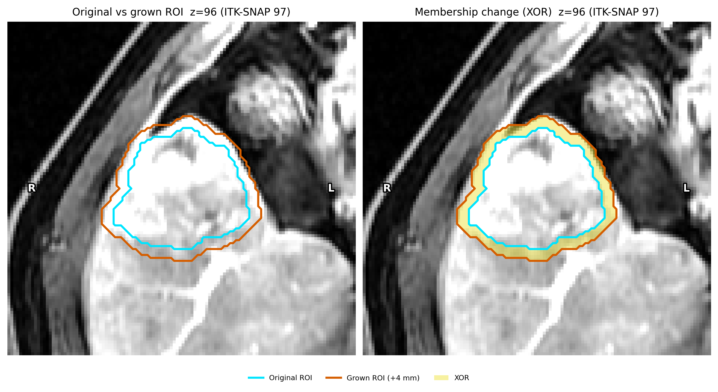
Uniform morphological grow of an ROI contour — `morphological_grow_shrink()` via the `morphological` registry name (grow +4 mm). Same PNG as the gallery script `contour_perturbation_demo.py`.

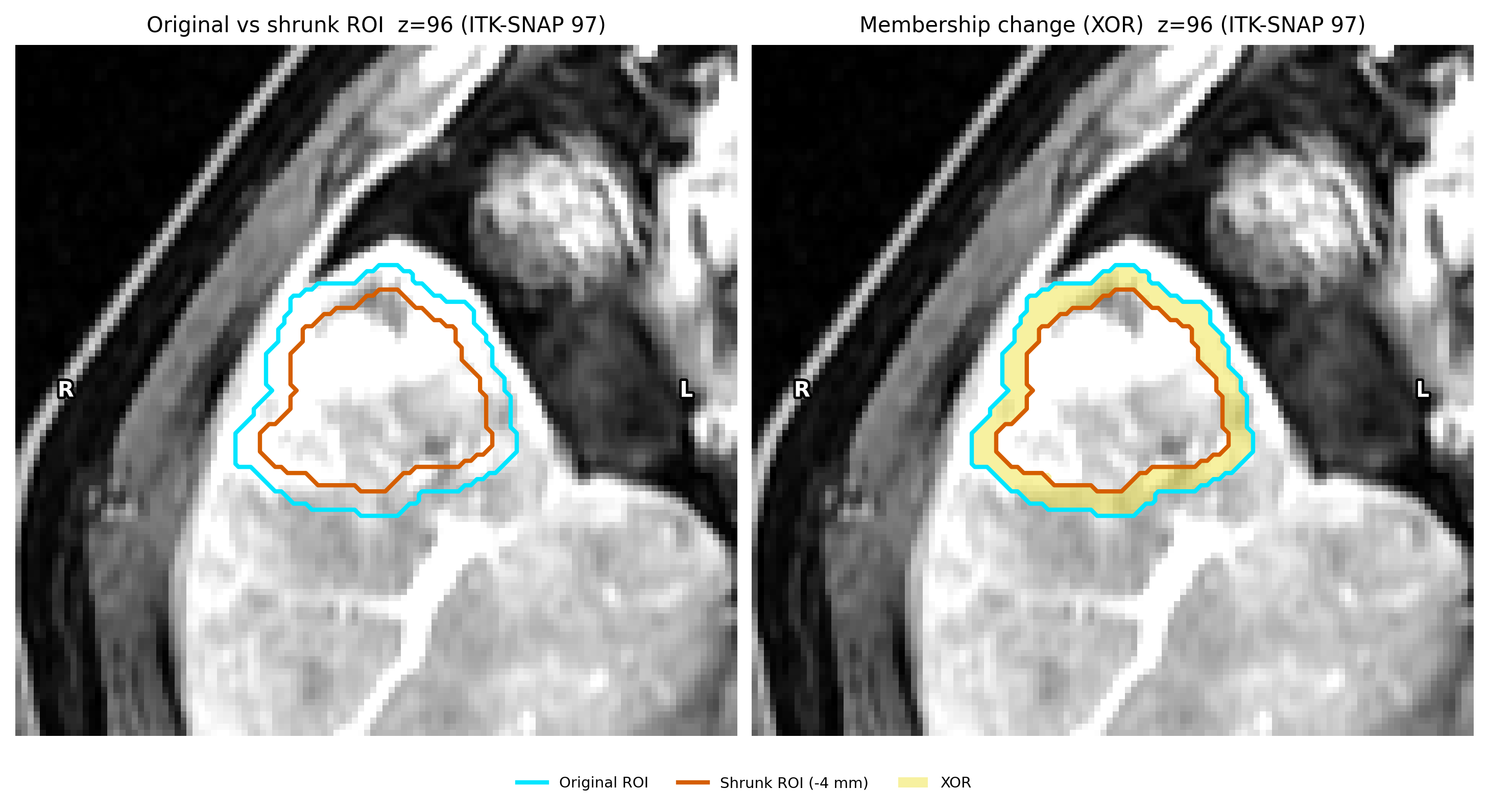
Uniform morphological shrink of an ROI contour — Same kernel, negative radius (shrink -4 mm).

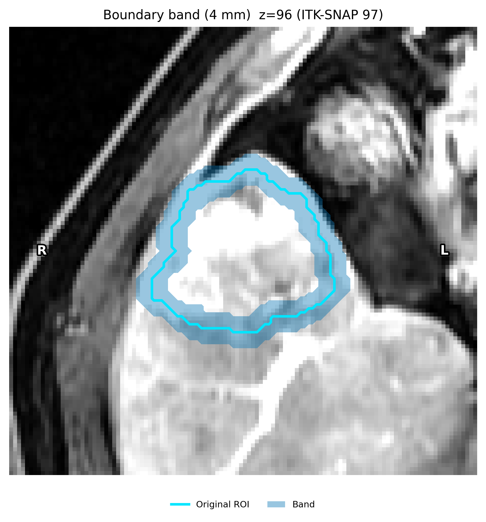
Boundary band around an ROI — `boundary_band_mask()` (4 mm half-width).

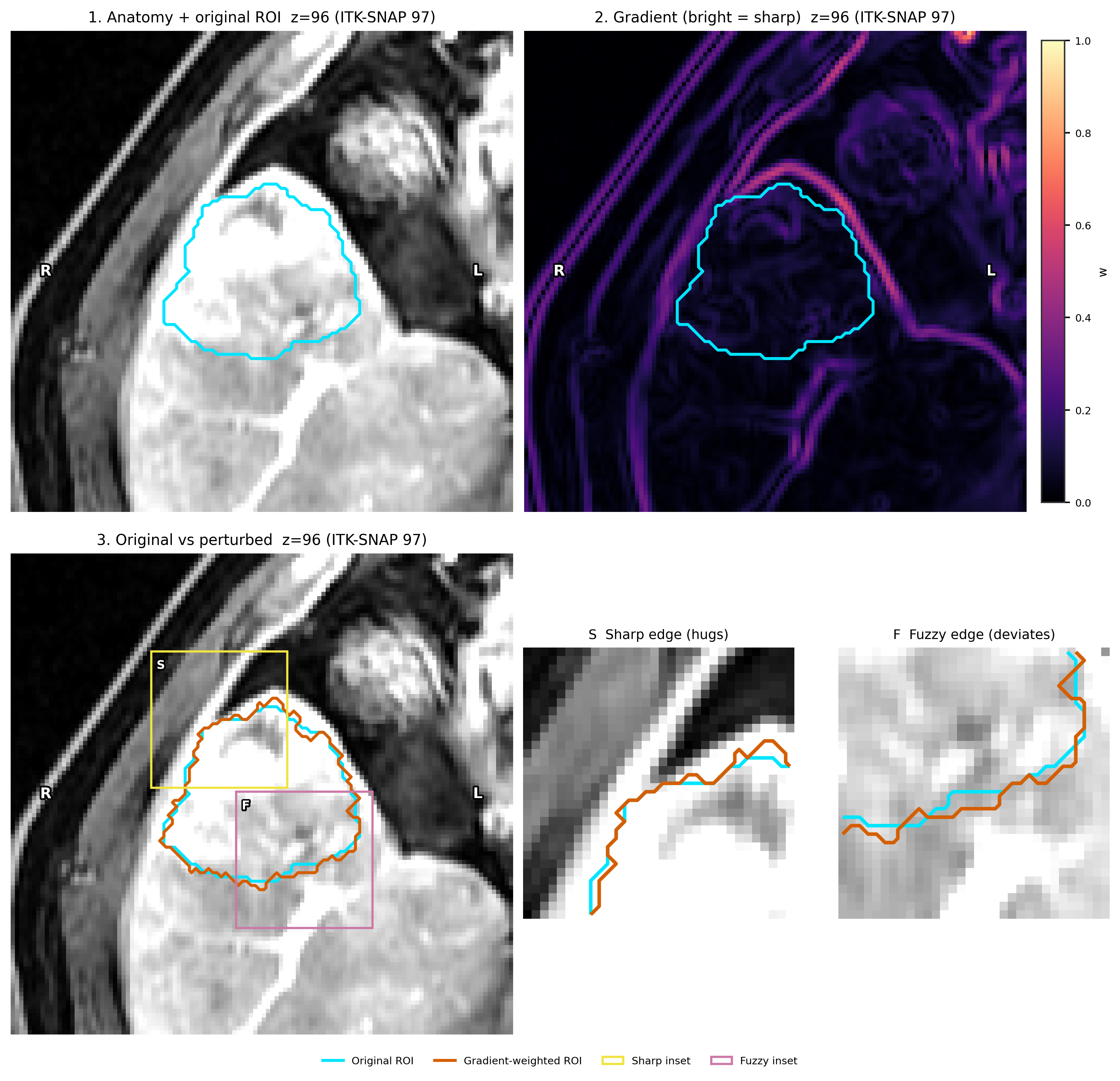
Gradient-weighted boundary perturbation — `boundary_weighted_perturbation()` via `gradient_weighted`. Anatomy, gradient (bright = sharp), cyan vs vermillion solid contours, plus sharp / fuzzy insets. Flip probability scales with `1 - normalised_gradient`.

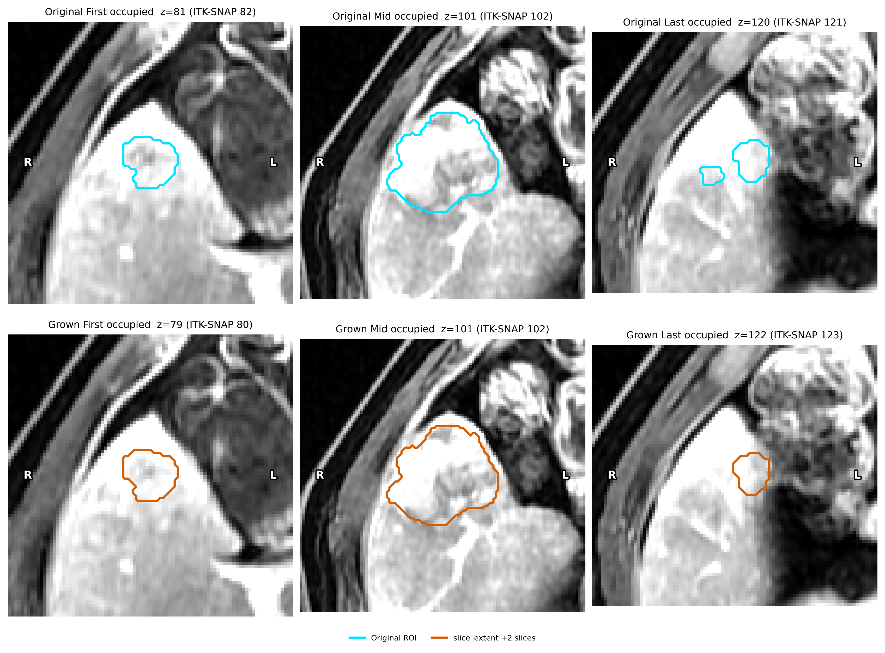
First mid and last slices after z-extent grow — `slice_extent_perturbation()` via `slice_extent` (`grow_slices=2`).

Classification statistics

midranks = compute_midrank(scores)
auc, var = fast_delong(predictions_sorted)
result = delong_roc_test(y_true, scores_a, scores_b)
ci = delong_roc_ci(y_true, scores)
var_ab = delong_roc_variance(y_true, scores_a, scores_b)
hl = hosmer_lemeshow_test(y_true, scores, n_groups=10)
sp = spiegelhalter_z_test(y_true, scores)

Habitat label matching

Independently clustered maps permute integer ids. Import the kernel directly (it is not re-exported from habit.kernels). There are two matchers, chosen by what the maps share:

overlap — the maps label the same voxels (observers, test–retest, perturbation, another preprocessing chain): Hungarian on voxel overlap, match_labels_by_overlap(). Domain wrappers: align_habitat_map(), habitat_stability().
prototypes — the maps label different patients: match_rows_to_prototypes() (K = largest habitat count, iterative assign / update, one habitat per prototype per subject). metric is "sqeuclidean" (default, mean update), "manhattan" (median), "cosine" or "correlation" (unit-vector mean); max_distance (off by default) allows partial assignment; prototypes= freezes a trained set. Two subjects are the special case of pairwise Hungarian on squared Euclidean distance. Rescale columns first with fit_feature_match_scale() when features have different units. Domain wrapper: align_habitat_maps_to_prototypes(). Method and references: Matching habitat labels across fits and subjects.

Copy-ready walkthrough: Match habitat ids.

from habit.kernels.habitat_label_match import (
    match_labels_by_overlap,
    match_rows_to_prototypes,
)

# Same tumour, two observers: overlap.
mapping = match_labels_by_overlap(physician2_labels, other_labels)

# Different patients: one (n_habitats, n_features) block per patient,
# habitat counts may differ. result.assignments[s][i] is the prototype
# index of habitat row i of patient s.
result = match_rows_to_prototypes([patient_a, patient_b, patient_c])

# A new patient named with the trained prototypes (no refit).
new = match_rows_to_prototypes([patient_d], prototypes=result.prototypes)

Stability

Published metrics (MSI, ITH, ICC, DeLong, Hosmer–Lemeshow, Spiegelhalter) are a stable subset within v1.x.

Numeric kernels (habit.kernels)